
This passage is my understanding of first 3 chapters of Introduction to Linear Algebra, and I will make some different on lecture sequence with MIT. Then maybe will tell something for previewing.
That’s all, let’s begin.
Vector
First, I will tell you what is vector and two operation with vector in Linear Algebra.
Basic Difinition
A vector would be written as below’s format,
For a vector named , it will be written as a column as order of it components from up to down, then enclose it in a square bracket. Denote it as in bold or under a right arrow.
OKay, that basic difinition of vector, also we have some special, a vector which all components are zero, such vectors we called zero vector denote as .
Then we have geometry meaning of vectors. For a vector with components, we believe that it is dimension. So we can draw it in a dimension space. For example, we can draw in a plane. (because of inline Latex require, I cannot type vector in column format, sorry.)
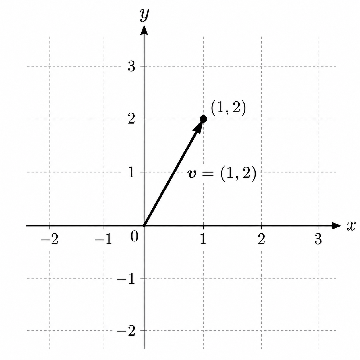
The drawing rule is find the point denotes vector then make a arrow from to point.
Basic Operations
Next, let we see two operation of vector in Linear Algebra: Scalar multiplication and addition. First is scalar multiply, most of number we studied in primary school is scalar like nature number, float, etc. That means scalar can multiply with a vector,
Then is vector addition, two vectors can be added when they have same component quantity, such as
Also we can understand these two operation in geometry meaning. Let me show you times when equal ; And add .
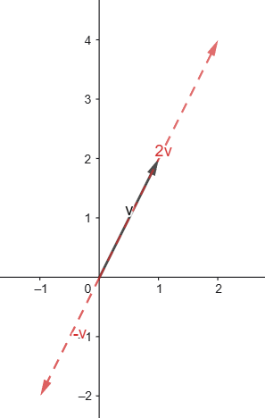
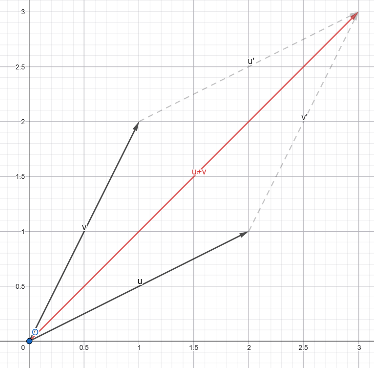
The second picture is vector addition, the parallelogram I drew is called parallelogram law, also we have triangle law, that all help us draw vector addition in space quickly. Just let these vector end-to-end connect the start point to the end point is answer vector. This is very important in next part.
Linar Combination
Now we know what is vector and two operation in Linear Algebra, now we can start to entrance the Linear Algebra world. The question you may ask naturally is, why these two operation? What will I get if I combine them?
So the Linear Combination going out naturally. For a group of , below formula called Linear Combination.
You can check can or cannot calculate all vector in plane by Linear Combination. Of course can, so the next part we are going to find some pattern in Linear Algebra.
Space
We use to denote all real numbers, and it is obviously 1 dimension. And is to denote a 2 dimension plane, is to denote a 3 dimension space, etc. These are all special space.
The definition of space is a set that the vector in space after linear combination are still in space, just like group. To understand it, I can give some example.
Such as, do you think is a space? No, because when , is not in space. It seems that single vector cannot form a space. No, zero vector can. Because whether what value takes.
That give out a tips: all space got in its dimension, that because when , all vector multiply become .
So this time we got smart, we can use all vectors on the line which through origin point and node , that must be a space. Why? Because you can find whether how we linear combination these vector they still on this line. This pattern stand in all dimension even 11 dimension, if only it a line through zero point, it is a space. Also we can generalize this property to spaces of other dimensions:
In a space, a set of -dimension vectors () through origin point form a space.
It could be a line through origin in , a plane through origin in , even whole (that is because through origin obviously)
Independence
Without zero vector, we expect vectors can span to a -dimension such as and zero vector can span to a 1 dimension line, and zero vector can span to a 2 dimension plane.
But there is a counterexample, or there are many conterexamples, for example and cannot span to a 2 dimension plane but a 1 dimension line. That shows a new pattern to us, we call this pattern as Independence.
The reason of and cannot span to a 2 dimension plane is . For a set of vector, if one of them can be denote by others linear combination, we call this vector is dependence with other vector. Or, we call this set of vector is independence.
There is a common mistakes: is not independ with any vectors.
Linear Basis
Ok, here is another new concept, because of in the example line through origin and , the vector obviously have strong connection with that space. The Linear Basis is coming out.
Why I always say span a space, span a space, that must because these vector have some significant connection with them space. The answer is, you can find that all vector in those space can be denoted by the linear combination of vectors I given.
The definition of Linear Basis is that a set of vectors which are independence. We call a basis of space is that a set of vectors which have minimum size and independence and it can span to the space. And obviously the basis of a space is commonly not unique.
Because is not independ with any vectors, so basis are always without zero vector, except a space only have zero vector.
The basis also have dimension, because of all vector in basis are independence, so the dimension of basis is the size of basis. Also we can optimize the definision of space: the dimension of space equal to the dimension of its basis.
In the following article, I will use to denote the dimension of .
Orthogonality
This part was written in book but MIT didn’t teach in the part which corresponding lecture. And it is also become a big nature when we are studing four subspace of matrix.
For two vectors in same dimension, we multiply each pair of components and sum them called dot product. And it is a scalar, below is a example:
And for a pair of special vectors, such as
We called , and this is orthogonality. If dot product answer of two vectors is zero, they are vertical.
Matrix
This part we are going to learn a new concept, Matrix. For a matrix which is , I will write it as below form, and denotes the element which place -th row and -th column.
Matrix also have two basic operation, and in this part we will learn it and use them analyze a classic problem in Linear Algebra next part.
Let’s begin.
Multiplication
The most important operation is Matrix Multiplication, we use below
to calculate it:
So it is not hard to find that the quantity of A’s column must equal to the quantity of B’s row. We usually say is a matrix, is a matrix. Basically, all the operation of matrix can be rewritten in a matrix multiplication form.
Because of the special calculate way of matrix multiplication, the matrix multiplication doesn’t support commutative law but it does support associative law. So we always multiply a matrix at left to find more connections:
Analogy scalar multiplication, maybe matrix multiplication also have a identity just like number , which can make every matrix multiply it will not change. Yes it is obviously have, we call this martix , identity matrix.
This matrix are written as a square matrix, and it is all zero but only main diagonal one. below is a identity matrix:
Matrix multiplication is a great operation, there are a further understanding of it, Linear Combination. We can only observe one process of multiplication in below example:
This is nothing news, right? But if I change the to one, the difference happened.
The first line of answer becomes sum of first line and last line of ! Why? Think the process of multiplication, you can find that when first row times each column of , we sum the first row element and last row element:
So we find the key, when we left times a matrix, the row of first matrix control the linear combination coefficient of second rows, that means answer matrix can write by below forms, denote the -th row of matrix .
That means left-multiplication denotes row of times each row of . Also we can check the similiar nature of right-multiplication. Observe below two expression:
Now the change happened on last column, and we can find the pattern easily by experience before, that is the linear combination coefficients of column of are depend on the columns in .
So we get the most important nature: left-multiplication controls row combination and right-multiplication controls column combination.
Inverse
Think the knowledge we learn in scalar multiplication, there is a concept just like reciprocal which satisfy , it called Inverse. We use to denote it. This will help us to derive expresion.
Now we don’t need to know how to calculate it but should know the concept. And not all the matrices can be inversed.
Transpose
Transpose a matrix follow rule , so the matrix will be transpose to a matrix. Below is two example:
And there also have a obviously pattern:
Also you just need to know a concept now, the applying will coming soon.
Permutation Matrix
After the matrix multiplication, there is a interesting operation is switching two row or two column of a matrix. Let us start with switching rows.
Because of the conclusion we find, we find that if we just need to switch two rows, we can just switch the corresponding row of identity matrix. For example, we need to switch the row and row of a matrix, so we do:
You know we have permutations of identity, for a identity these matrices called Permutation Matrix. This set of matrices also make up a group about operation transpose (or inverse).
Below is all permutation matrix which is .
The transpose of them is:
It is obviously same because set is unordered. So that is why I say these permutation make up a group with operation transpose. But why I also say they make up with inverse? Now let’s prove a scary theorem: .
The first row will transpose to first column and second row will transpose to second column, but just when same row times same column it will get one, so that means only will have one, it is a identity matrix. Q.E.D.
Now we are know all the opertion of matrix, next part we are going to solve a classic problem and leading out the most important concept in linear algebra.
Elimination
This part is to lead out the most important concept through a classic problem in Lienar Algebra. The classic problem is Elimination, Gauss gave us a algorithm to solve it. We can find the four subspace of a matrix from it.
Pivot
The first things is that elimination seems equations and unknowns problem, why it can be solved by matrix? Let’s begin with a three equations and three unknowns problem.
This cases can be rewritten in below matrix expression
Check it by yourself. In following article, I will call the first martix , the second matrix(or vector) , and the answer matrix(or vector) . So the equation is in form . Because of I said right multiplication depend the linear combination coefficient of , so we also can write it in below form:
It seems that those column vectors span a space, this space is called Column Space, denote as , so we know has solution when . The dimension of this space we can know from elimination process.
Now let me tell you the algorithm process of Gauss’ algorithm. First we find a Pivot, pivot cannot be zero because zero cannot use to eliminate other rows. Then use pivot let the rows below become zero. That’s all, try it. Oh, you also should put the matrix after , let change with elimination, we call this matrix Augmented Martix.
Pivot cannot be zero, switch the row one and two.
Minus row three with two times of row one.
Minus row three with 3/2 times row two.
Now we get three pivot, this means that we have three indenpendence columns, so the is span to a 3-dimension space. The quantity of pivot we called rank denoted as , so obviously that .
And the left part of this matrix called up triangluar matrix, denote as .
The following operation of elimination is back substitution. We found that the last row we have , so we can know that , then back substitute this value to second row, then get .
That is the all process of Gauss’ Algorithm.
Column Space
Now we have finished the basic process of elimination, let us go back to the concept we found before, Column Space.
We know when a matrix is
and a vector is
we have known from Matrix Multiplication part that
That means the answer of is just a Linear Combination of columns in . So when can take all possible value, all possible answer of will span to a space, we call this space Column Space, denote as .
So we can write
Also we can write it in another form
These two forms are same. First one view it from Linear Combination, second one view it from matrix multiplication.
There is a thing should notice. If is a matrix, the columns of have components, so those vectors are in . That means
But have components, so is in . We can write the whole process like
This pattern will be important when we learn other three spaces, remember it.
Now come back to equation . Because can only be the Linear Combination of columns in , if is not in , there is obviously no can let . So has solution only when is in . That means solving a equation also have a geometry meaning: we are checking whether is in the space which columns of span.
Then here is another question. Do all columns in are useful to span ? Of course not, because we have learned Independence before, For example
There are three columns
But , So is not independence with first two columns, remove it will not change .
We need find a basis of , and the answer have already appeared in Elimination: Pivot Column.
If after elimination the pivot appear at column , that means the column are independence with each other and other columns can be Linear Combination from them. So these columns make up a basis of .
But there is a common mistake: we should take column from original matrix , not from the matrix after elimination. Because row operation will change columns, so generally .
Elimination just tell us which column position are pivot, then we go back to original to get them.
Now remember the definition of rank before. Rank is the quantity of pivot, and now pivot columns form a basis of . The dimension of a space is the size of its basis, so we get .
That give out a more important meaning of rank. Rank is not just how many pivot we find, it is also how many independence directions this matrix columns can give.
For a matrix whose columns are in , if , then is a line through origin. If , then is a plane through origin. And if , then . I already said it before, it is the geometry meaning of rank.
Because is in , its dimension cannot bigger than , and because only have columns, it also cannot bigger than . So .
Inverse
We have already known the basic concept of Inverse in Matrix part. Now after Elimination, we can use it to calculate inversre of a matrix. Why inverse is useful? Look at equation . If exist, we can left multiply on both side . Because , we get . So inverse can directly give out the answer of equation.
But not all square matrix can be inversed. Now Rank can tell us when it can.
For a matrix, if then it have pivots, so elimination can finally change into . Also from Column Space we know every have solution when .
And because every column have pivot, there will be no free variable, so every also have only one solution.
We can also use Elimination to calculate inverse.
Think we want find a matrix satisfy . If we use row operations change to , all those row operations together are exactly changing to . So we put after just like Augmented Matrix in Gauss’ Algorithm. For example, start with
Minus row two with three times row one
Divide row two by
Minus row one with two times row two
So
You can multiply to check it by yourself. Now there is a interesting question: we said every row operation can be described by left multiplication, so can we write every step of Elimination as a matrix?
Of course can, that is next concept.
Elimination Matrix
We have learned before that left-multiplication control the rows of matrix. So every row operation in Elimination can also be written as left multiply a matrix. We call such matrix Elimination Matrix. For example,
To eliminate , we need , from left-multiplication part, we know that we can change the second row of to coefficients we want
Then
So just finish the row operation.
If we have many elimination operations, we have many Elimination Matrices
and the whole elimination process can write as
There is another easy pattern. Because makes , its inverse should make , so
In this simple elimination matrix, inverse just change the sign of number below diagonal. This connection is very important because now we can rewrite the whole elimination process backward.
And that will give out LU Factorization.
PA = LU
We have the elimination form with elimination matrix. Left multiply inverse matrices in reverse order, we get
Let
then
This is called LU Factorization, is for Lower Triangular Matrix.
Let us do a example
First eliminate first column, and . Then eliminate second column , Finally we get
The multipliers we used are , put them into the positions below diagonal, then we get
And we can check . This is a very useful way to remember : the number we used to eliminate each position can directly put into corresponding position of .
But there is one problem. What if elimination need switch row?
You can remember the example we used before, its first pivot is zero, so we switched row one and row two. Row switching is not an elimination matrix, we have already made a special matrix for it: Permutation Matrix.
So if row switching happened, generally we use , that is called PLU Factorization.
Now we have almost finished the calculation side of elimination. Let us come back to , because it will give out the second space of .
Null Space
Before we always solve , now let become zero vector . The set of all which satisfy this equation is called Null Space, denote as . That means .
Notice the difference with Column Space. If is a matrix, Column Space is in , but have components, so . That means Column Space and Null Space are even not in same whole space generally.
Let us find a example which have non-zero vector in Null Space
We eliminate it
There are two pivots, we have variables, but just pivot variables. So the other two variables are free variables. Let , back substitution. From second row , so . From first row , so . Then all solution can write as
Use linear combination to write this expression,
So
These two vectors are independence, so they form a basis of .
We have columns and pivots, so there are free variables. Every free variable give out one special solution, so . This formula is very important.
There is also a useful nature from Elimination. Row operations do not change solution of , or elimination become wrong. It means that row elimination will not change Null Space, so .
That is different with Column Space. We have learned row operation usually change , but it does not change .
But a matrix actually have four important spaces. To find another two, we need use Transpose we have introduced before.
Four Subspaces
This part I will tell all the subspaces of matrix and show there connections.
Column Space of Transpose
We have already learned Transpose before. For a matrix , is a matrix. Of course have its Column Space . But columns of are rows of after we write them as column vectors. So is also called Row Space of .
For example
then
So
But second vector is two times first vector, so this row space are a line through origin.
Now there is a very important theorem: . Becasue transpose obviously don’t change the pivot quantity when Elimination, and also row operations do not change .
If is , every row of have components, so . This is same whole space with .
It seems that has more connection with .
Null Space of Transpose
Now just like what we did before, also have a Null Space . Its definition is , because is , the vector have components, so . This is same whole space with .
We can find its dimension using same formula of Null Space. The rank of is also , and have columns, so So now we finally have all four spaces, .
Let us use the matrix in Null Space example again
We know rank of this matrix is two, and is , so , , , . We can also calculate last space directly.
Because third row of is first row plus second row, if
then
So
Now the last thing we need is put these four spaces together.
Four Fundamental Subspaces
We have found four spaces from one matrix
They are called Four Fundamental Subspaces.
We can summarize all things into below table:
| Space | In | Dimension | Meaning |
|---|---|---|---|
| All possible output of | |||
| Input which change to zero | |||
| Space spanned by rows of | |||
| Vectors orthogonal with Column Space |
But the connection is not just their dimensions add to whole space. Remember the Orthogonality we learned in Vector part. Take any , then .
What does this equation mean by rows? Every row of dot product with equal zero. So is orthogonal with every row of , and of course also orthogonal with every Linear Combination of rows. But all Linear Combination of rows make up . So .
And because their dimensions together equal , they fill the whole .
So
Same pattern happened in .
and their dimensions together equal , so
The here means every vector in the space or can be describe by linear combination of a pair of vectors in each space.
Now we can finally understand the four rectangles diagram in Linear Algebra.
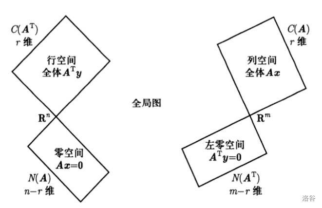
The left whole space is . It contains and . The right whole space is . It contains and . Also the two pair of spaces are orthogonal, that why these irregular quadrilateral seems vertical on their intersection
That’s all, thanks for reading.